
Solving Block World Search Nov. 26, 2015 in Algorithms, Java, Text, University
Block world is a simple 2D sliding puzzle game taking place on a finite rectangular grid. You manipulate the world by swapping an agent (In this case the character: ☺) with an adjacent tile. There are up to 4 possible moves that can be taken from any tile. As you can imagine, with plain tree search the problem quickly scales to impossibility for each of the blind searches.
It is very similar to the 8/15 puzzles, just with fewer pieces, meaning it’s simpler for the algorithms to solve. It’s unlikely any of my blind searches could solve a well shuffled tile puzzle with unique pieces, but I suspect my A* algorithm could. However, before doing so I would want to spend time improving my Manhattan distance heuristic, so it gave more accurate results over a larger range.
I decided to use Java to solve this problem, as I’m familiar with it and it has a rich standard library containing Queue, Stack, and PriorityQueue. These collections are vital to implementing the 4 search methods. You can implement the different searches differently, but the data structures I listed just deal with everything for you.
Search Methods
To solve the block world problem, I implemented three blind tree searches and a single tree heuristic search. Additionally, I can pass a single parameter to each search which checks if the grandparent state and the child state are identical, now it’s a very simple graph search. This single calculation performed once per node expansion significantly reduces the time and space complexity. It’s not perfect as it is still possible to visit states twice, it just takes longer to do so; a better solution would store a set of visited states.
Breadth First Using a queue, poll it and check if it has reached the goal. If not, expand, and add the children back to the queue. This search is both complete and optimal, but slow and memory intensive, as you need to keep every node in memory.
Depth First Using a stack, take the top node of the stack, and check if it has reached the goal. If not expand, shuffle the children and add them back to the stack. This search is neither complete nor optimal and produces rather terrible solutions. Without shuffling, infinitely looping is likely.
Deepening Using Depth First Search, give the blind search an incrementing limit which it fully explores until it finds the goal. This search is both complete and optimal. Better memory usage than breadth first search - you don’t need to keep every node in memory.
A* Heuristic Using a priority queue, poll it and check if it has reached the goal. If not expand, use a heuristic to guess the final cost of each child and add the children back to the queue. If the heuristic is admissible, i.e. is optimistic and never overestimates, then the solution is complete, optimal and fast. I use Manhattan distance divided by two for my heuristic. I divide by two because swapping the tiles moves two tiles and could conceivably lead to a situation where the heuristic over estimates, by double. This does however slow the search down.
Implementation
I defined an abstract class Search and an interface Heuristic, too allow me to pass any searching algorithm or heuristic to a general expansion function. All my searching algorithms are implemented using these. This helps to minimize the coupling between different classes. In addition, I have a helper class Position2D and three more important classes: Simulation, Node, and State. Simulation keeps track of the outputs of each search, and runs the program; Node deals with the tree structure and manipulating it; and State contains the programs state. Each class knows as little as possible about each class.
Operation
Below is my Program in operation on the example given which has a depth of 16. For speed I used A* Search to generate the following paths, although that doesn’t really matter as any optimal search should arrive at the same solution, or at least arrive at a solution of identical depth:
| Start | ↑ | ← | ↓ | ← | ← | ↑ | → | ↓ | → | ↑ | ↑ | ← | ↓ | ↓ | → | → |
|---|---|---|---|---|---|---|---|---|---|---|---|---|---|---|---|---|
| ␣␣␣␣ | ␣␣␣␣ | ␣␣␣␣ | ␣␣␣␣ | ␣␣␣␣ | ␣␣␣␣ | ␣␣␣␣ | ␣␣␣␣ | ␣␣␣␣ | ␣␣␣␣ | ␣␣␣␣ | ␣␣␣␣ | ␣␣␣␣ | ␣␣␣␣ | ␣␣␣␣ | ␣␣␣␣ | ␣␣␣␣ |
| ␣␣␣␣ | ␣␣␣␣ | ␣␣␣␣ | ␣␣␣␣ | ␣␣␣␣ | ␣␣␣␣ | ␣␣␣␣ | ␣␣␣␣ | ␣␣␣␣ | ␣␣␣␣ | ␣␣␣␣ | ␣␣☺␣ | ␣☺␣␣ | ␣A␣␣ | ␣A␣␣ | ␣A␣␣ | ␣A␣␣ |
| ␣␣␣␣ | ␣␣␣☺ | ␣␣☺␣ | ␣␣C␣ | ␣␣C␣ | ␣␣C␣ | ☺␣C␣ | ␣☺C␣ | ␣AC␣ | ␣AC␣ | ␣A☺␣ | ␣A␣␣ | ␣A␣␣ | ␣☺␣␣ | ␣B␣␣ | ␣B␣␣ | ␣B␣␣ |
| ABC☺ | ABC␣ | ABC␣ | AB☺␣ | A☺B␣ | ☺AB␣ | ␣AB␣ | ␣AB␣ | ␣☺B␣ | ␣B☺␣ | ␣BC␣ | ␣BC␣ | ␣BC␣ | ␣BC␣ | ␣☺C␣ | ␣C☺␣ | ␣C␣☺ |
And here is it in reverse problem, also of depth 16:
| Start | ← | ← | ↑ | ↑ | → | ↓ | ↓ | ← | ↑ | ← | ↓ | → | → | ↑ | → | ↓ |
|---|---|---|---|---|---|---|---|---|---|---|---|---|---|---|---|---|
| ␣␣␣␣ | ␣␣␣␣ | ␣␣␣␣ | ␣␣␣␣ | ␣␣␣␣ | ␣␣␣␣ | ␣␣␣␣ | ␣␣␣␣ | ␣␣␣␣ | ␣␣␣␣ | ␣␣␣␣ | ␣␣␣␣ | ␣␣␣␣ | ␣␣␣␣ | ␣␣␣␣ | ␣␣␣␣ | ␣␣␣␣ |
| ␣A␣␣ | ␣A␣␣ | ␣A␣␣ | ␣A␣␣ | ␣☺␣␣ | ␣␣☺␣ | ␣␣␣␣ | ␣␣␣␣ | ␣␣␣␣ | ␣␣␣␣ | ␣␣␣␣ | ␣␣␣␣ | ␣␣␣␣ | ␣␣␣␣ | ␣␣␣␣ | ␣␣␣␣ | ␣␣␣␣ |
| ␣B␣␣ | ␣B␣␣ | ␣B␣␣ | ␣☺␣␣ | ␣A␣␣ | ␣A␣␣ | ␣A☺␣ | ␣AC␣ | ␣AC␣ | ␣☺C␣ | ☺␣C␣ | ␣␣C␣ | ␣␣C␣ | ␣␣C␣ | ␣␣☺␣ | ␣␣␣☺ | ␣␣␣␣ |
| ␣C␣☺ | ␣C☺␣ | ␣☺C␣ | ␣BC␣ | ␣BC␣ | ␣BC␣ | ␣BC␣ | ␣B☺␣ | ␣☺B␣ | ␣AB␣ | ␣AB␣ | ☺AB␣ | A☺B␣ | AB☺␣ | ABC␣ | ABC␣ | ABC☺ |
Randomly generated problem of depth 16, I chose 16 so it’s easier to compare. Any number could be picked.
| Start | ← | ← | ↑ | → | ↑ | ↑ | ← | ↓ | ↓ | → | ↑ | ↑ | ← | ↓ | ← | ↓ |
|---|---|---|---|---|---|---|---|---|---|---|---|---|---|---|---|---|
| A␣␣␣ | A␣␣␣ | A␣␣␣ | A␣␣␣ | A␣␣␣ | A␣␣␣ | A␣☺␣ | A☺␣␣ | AB␣␣ | AB␣␣ | AB␣␣ | AB␣␣ | AB☺␣ | A☺B␣ | ACB␣ | ACB␣ | ACB␣ |
| ␣B␣␣ | ␣B␣␣ | ␣B␣␣ | ␣B␣␣ | ␣B␣␣ | ␣B☺␣ | ␣B␣␣ | ␣B␣␣ | ␣☺␣␣ | ␣C␣␣ | ␣C␣␣ | ␣C☺␣ | ␣C␣␣ | ␣C␣␣ | ␣☺␣␣ | ☺␣␣␣ | ␣␣␣␣ |
| ␣␣C␣ | ␣␣C␣ | ␣␣C␣ | ␣☺C␣ | ␣C☺␣ | ␣C␣␣ | ␣C␣␣ | ␣C␣␣ | ␣C␣␣ | ␣☺␣␣ | ␣␣☺␣ | ␣␣␣␣ | ␣␣␣␣ | ␣␣␣␣ | ␣␣␣␣ | ␣␣␣␣ | ☺␣␣␣ |
| ␣␣␣☺ | ␣␣☺␣ | ␣☺␣␣ | ␣␣␣␣ | ␣␣␣␣ | ␣␣␣␣ | ␣␣␣␣ | ␣␣␣␣ | ␣␣␣␣ | ␣␣␣␣ | ␣␣␣␣ | ␣␣␣␣ | ␣␣␣␣ | ␣␣␣␣ | ␣␣␣␣ | ␣␣␣␣ | ␣␣␣␣ |
And it’s reverse, note the path taken is different, but of the same depth:
| Start | ↑ | → | ↑ | → | ↓ | ← | ↓ | → | ↑ | ← | ↑ | → | → | ↓ | ↓ | ↓ |
|---|---|---|---|---|---|---|---|---|---|---|---|---|---|---|---|---|
| ACB␣ | ACB␣ | ACB␣ | A☺B␣ | AB☺␣ | AB␣␣ | AB␣␣ | AB␣␣ | AB␣␣ | AB␣␣ | AB␣␣ | A☺␣␣ | A␣☺␣ | A␣␣☺ | A␣␣␣ | A␣␣␣ | A␣␣␣ |
| ␣␣␣␣ | ☺␣␣␣ | ␣☺␣␣ | ␣C␣␣ | ␣C␣␣ | ␣C☺␣ | ␣☺C␣ | ␣␣C␣ | ␣␣C␣ | ␣␣☺␣ | ␣☺␣␣ | ␣B␣␣ | ␣B␣␣ | ␣B␣␣ | ␣B␣☺ | ␣B␣␣ | ␣B␣␣ |
| ☺␣␣␣ | ␣␣␣␣ | ␣␣␣␣ | ␣␣␣␣ | ␣␣␣␣ | ␣␣␣␣ | ␣␣␣␣ | ␣☺␣␣ | ␣␣☺␣ | ␣␣C␣ | ␣␣C␣ | ␣␣C␣ | ␣␣C␣ | ␣␣C␣ | ␣␣C␣ | ␣␣C☺ | ␣␣C␣ |
| ␣␣␣␣ | ␣␣␣␣ | ␣␣␣␣ | ␣␣␣␣ | ␣␣␣␣ | ␣␣␣␣ | ␣␣␣␣ | ␣␣␣␣ | ␣␣␣␣ | ␣␣␣␣ | ␣␣␣␣ | ␣␣␣␣ | ␣␣␣␣ | ␣␣␣␣ | ␣␣␣␣ | ␣␣␣␣ | ␣␣␣☺ |
As you can see, my solution not only can generate random problems, but solve them optimally. Just for fun, here is Depth First Search on the top problem. It only took 1687 steps, which is low for Depth First Search:
▲◀◀▼◀▲▲▲▶▼▶▲▶▼◀▼▼◀▲▶▶▲◀▼▶▲▲◀▼▶▲◀▼▼▶▼◀▲◀▲▶▼▶▲▲◀▼▼▼◀◀▲▶▼◀▲▲▲▶▶▶▼▼◀▲▲◀▼▶▼▼▶▲◀▼▶▲◀▲▶▲◀▼▶▼▼◀▲▲▲◀◀▼▶▲▶▶▼▼▼◀◀◀▲▲▶▼◀▲▲▶▶▼▼▼▶▲▲◀▼▼▶▲◀▲▶▼◀▲◀▲▶▼◀▲◀▼▶▲◀▼▼▼▶▲◀▼▶▲▶▲◀▲▶▼◀▲◀▼▶▼◀▲▲▶▶▶▼◀▼▶▼◀▲▲▶▲◀▼◀◀▼▼▶▲▲◀▲▶▶▶▼◀▲◀▼▶▲◀▼◀▲▶▶▶▼◀▼▶▼◀◀◀▲▶▼◀▲▲▶▶▶▼◀▼▶▲▲◀▲▶▼◀◀◀▲▶▶▶▼▼◀◀▼▶▲◀▼▶▲◀◀▲▶▼▼◀▲▲▶▶▲◀◀▼▼▼▶▲◀▼▶▲◀▲▶▼▼◀▲▲▲▶▼◀▲▶▼◀▲▶▼▶▼▼◀▲▲▶▼▶▲▲◀◀▼▶▼◀◀▼▶▶▶▲◀◀▲◀▼▼▶▲▲▶▶▼▼◀◀◀▲▶▶▼▶▲◀▼◀◀▲▲▶▶▶▼◀◀▲▶▼▼◀◀▲▶▼▶▲▲▶▲◀▼▼▶▲◀▲▶▼◀▲▶▼▼◀◀▼◀▲▲▶▼◀▲▶▶▶▼▼◀◀◀▲▲▶▼▶▲▲▶▼▼◀▼▶▲◀▲◀▲◀▼▼▶▼▶▲◀▲◀▼▶▶▼◀▲◀▼▶▶▲◀▼◀▲▲▲▶▼▼◀▼▶▶▶▲◀▼▶▲▲◀◀▼◀▲▶▼▶▼◀◀▲▶▶▲▲◀◀▼▶▶▼◀▼▶▲▲▲◀◀▼▶▲◀▼▶▲▶▼◀▲▶▶▼▼◀◀▲◀▲▶▶▼◀▲◀▼▼▶▲▲◀▼▶▶▶▲◀▼▶▼▼◀◀▲◀▼▶▶▲◀▼▶▲▶▲◀▲▶▼◀▲◀▼▶▶▼◀▼▶▲▲◀▼▼▶▲▲▲◀◀◀▼▼▶▼▶▶▲▲▲◀◀◀▼▼▼▶▶▲▶▼◀▲▶▼◀◀▲▲▶▶▼◀◀▲▲◀▼▼▼▶▶▶▲▲▲◀◀▼▶▼▶▲◀▼◀▲▲◀▼▼▼▶▲◀▼▶▶▲▲◀▲▶▶▼▼▼◀▲◀▲▲◀▼▼▶▼▶▶▲▲▲◀▼◀▼▶▼◀▲◀▼▶▲▲▶▼▼◀▲▲▶▶▲◀▼▼▶▲◀◀▲◀▼▼▶▲◀▼▼▶▲▲▲◀▼▶▶▶▲◀▼▶▼◀◀▲▶▼▼◀▲▲◀▼▼▶▶▲◀◀▲▲▶▼▼◀▲▲▶▶▼▼▶▼◀◀◀▲▲▲▶▼▼▼▶▲◀▲▶▲▶▼◀▼◀▼▶▶▲◀◀▲▶▲◀▼▼◀▲▲▶▶▼▼▶▲▲◀▼◀▲▶▶▼▼◀◀◀▲▲▶▶▼◀▼▼◀▲▲▲▶▼▶▲▶▼◀▲◀▼▼▶▶▲◀◀▲▶▼▼▶▲▲◀◀▼◀▲▶▶▶▼▼◀▼◀◀▲▲▲▶▼▶▼▼◀▲◀▲▲▶▼▶▼▶▼◀◀◀▲▲▲▶▶▶▼▼◀◀◀▲▶▶▲▶▼▼▼◀◀▲▶▼◀▲▶▶▼◀◀◀▲▶▼◀▲▶▶▼▶▲◀◀▼▶▶▲▲◀▲◀▼◀▲▶▼▶▶▼▼◀▲▲◀▲▶▶▼▼◀▼▶▲▲◀▲▶▼▼▼◀◀▲▲▶▼▶▲▲◀◀◀▼▶▲▶▼◀▼▼▶▲▶▲◀▼▼◀▲▲▲◀▼▶▶▼▶▲◀▼▶▼◀◀▲◀▲▶▲▶▼▼▼◀▲▲◀▲▶▼◀▼▼▶▶▶▲◀▼▶▲▲▲◀▼▼◀▲▲▶▶▼▼◀▼◀▲▶▶▼◀▲▲▲▶▼◀▲◀◀▼▼▶▲◀▼▼▶▲◀▲▲▶▶▼▶▲◀▼▶▲◀◀◀▼▶▲▶▶▼◀▲▶▼◀▲◀◀▼▼▼▶▶▶▲◀▼◀▲◀▼▶▶▶▲◀▼▶▲▲◀◀◀▲▶▶▶▼▼◀▼◀◀▲▲▲▶▼▶▼◀▼◀▲▲▲▶▼▶▶▼◀◀▲▲▶▼◀▼▼◀▲▲▶▶▼◀▲▶▼◀▲◀▲▶▶▼◀◀▲▶▶▼▼▶▼◀▲▲◀◀▲▶▶▼▼▶▼◀◀▲▲◀▼▼▶▶▲▶▲◀▼▶▲▲◀▼◀◀▼▶▼◀▲▶▲▶▶▲◀▼▶▲◀▼◀◀▼▶▶▼◀▲▶▼▶▲▲◀▼▼▶▲◀◀▲▶▲◀◀▼▼▶▲▲▶▼▼▼◀▲◀▲▲▶▼▶▲◀◀▼▼▶▲◀▲▶▼◀▼▼▶▶▶▲◀▼◀▲◀▼▶▲▶▶▼◀◀◀▲▶▶▶▼◀▲▲▶▼◀▲▲▶▼▼◀◀▲◀▲▶▼▼▶▶▲▲◀◀▼▶▼▼▶▲▲▲◀▼▶▼▼◀◀▲▲▶▶▲◀▼◀▼◀▼▶▶▶▲◀▲◀▲▶▼◀◀▲▶▶▶▼◀◀◀▼▶▶▶▲◀▲◀▼▶▲◀▼▶▲▶▼◀◀◀▼▶▼◀▲▲▶▶▼◀◀▼▶▶▲▲▶▲◀▼▼▼◀◀▲▶▼◀▲▲▲▶▼▼◀▼▶▲▶▼▶▲◀◀◀▲▲▶▼◀▲▶▼▶▼▶▲◀◀▲◀▼▼▶▲▶▲◀◀▼▼▼▶▲◀▲▲▶▶▼◀▲◀▼▼▼▶▲▲▶▲◀▼◀▼▶▶▲▲▶▼▼▼◀▲◀▲▲▶▼▶▼▼◀▲▶▼◀▲▲▶▲◀▼◀▲▶▶▼▼▼◀▲▶▲▲◀◀▼◀▲▶▼▶▶▲◀◀◀▼▼▶▶▲▲▶▼▼◀▲◀◀▼▶▶▲▶▲◀◀▼▼◀▲▲▶▶▼▼▼▶▲▲◀▲◀▼▼▼◀▲▶▶▶▲◀▲◀◀▼▶▶▶▼▼◀◀▲▲◀▼▼▶▶▶▲▲◀◀▼▼▶▶▲◀◀◀▲▲▶▼▼◀▼▶▶▶▲◀▲▶▼▼◀▲▲▶▼◀▲▶▼◀▲▲▶▼◀◀◀▲▶▼▶▲▶▼▼▼◀▲▲▲▶▼▼▼◀▲◀▲▲▶▼▼▶▼◀▲◀▲▶▼▶▼
To (hopefully) make it easier to look at, I replaced the arrows with triangles, it’s clear depth first is terrible.
Scaling difficulty
I scaled the difficulty by taking a single start state: (“A␣␣␣”, “␣B␣␣”, “␣␣C␣”, “␣␣␣☺”) and randomly mutating it many times. As I varied the number of mutations, I would get problems of greater depth. I start with a small number of mutations, and as the program progresses, I slowly ramp it up. To get a good comparison, I run each problem with each search method multiple times, recording the average.
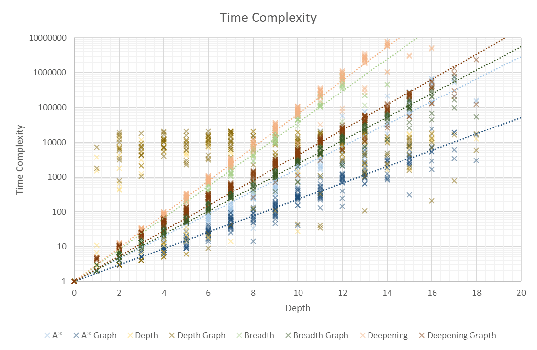
This method isn’t perfect as you can easily end up near the initial state regardless of how many mutations you perform. To combat this, I take the depth from one of my complete methods and use that to plot depth vs. time complexity. As a result, I get significantly more data points for smaller numbers and I cannot guarantee that every depth will be visited.
Results
Conclusions
Scalability
| Time Complexity | Space Complexity |
|---|---|
| 1. A* Graph Search | 1. A* Graph Search |
| 2. A* Search | 2. Iterative Deepening Graph Search |
| 3. Breadth First Graph Search | 3. A* Search |
| 4. Iterative Deepening Graph Search | 4. Breadth First Graph Search |
| 5. Breadth First Search | 5. Iterative Deepening Search |
| 6. Iterative Deepening Search | 6. Breadth First Search |
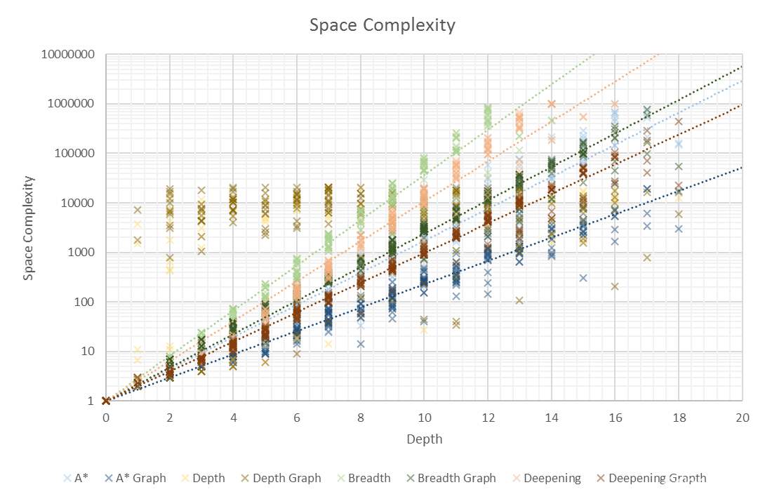
In both time and space, A* is in the lead. Iterative Deepening Search has terrible time complexity, but second-best space complexity. Breadth First Search performs badly, compared to the other searches. Treating the problem like a graph provides huge performance increases all around.
Algorithms
Breadth First Search is a pretty decent search algorithm for small problems, unfortunately it requires a lot of memory and quickly gets out of hand. However, the solutions found are both optimal and complete, it’s also easy to implement. It has better time complexity than Iterative Deepening
Depth First Search is terrible, while it may not look so on the graphs above, the reason is that towards the end, it usually wouldn’t find a solution without going over the limit I set, of a maximum of 1,000,000 nodes space complexity. Past a depth of about 10-15, many searches simply timed out leaving you with the lucky searches which completed. Therefore, I didn’t show a trend line for this search, it would be terribly subjected to survivorship bias.
Iterative Deepening Search is simple to implement on top of Depth First search and get good solutions. The upside is better space complexity, at the cost of time complexity. Due to how quickly you end up using gigabytes of memory even on a modern machine, this makes Iterative Deepening Search the second-best algorithm I implemented. It’s easier to wait longer than add more memory
A* Search is significantly better than any of the blind searches. This makes sense as it heuristically evaluates each child to priorities the node with the smallest estimated cost. Harder to implement than a blind search, and I don’t think my heuristic of simple Manhattan distance is very good. A* is only as good as its heuristic. A* with a bad heuristic is just Breadth First Search
Even the extremely crude graph search I implemented it improved every single search method. I have learned that when graph search is an option, it’s usually significantly faster than plain tree search, as you don’t need to visit the same states multiple times during each search. You can find a solution to the example question with Breadth First Graph Search, you can’t with Breadth First Search.
Limitations and Evaluation
As the solution becomes more complex, the only search that can keep up is A* search. In addition, Depth First Search is far too random and likely to fail for most practical applications.
Overall, I am pleased with my results, they clearly show the how time and space complexity vary with problem depth, even if the highest depth I go up to is around 20.