Machine Learning with MATLAB | Matthew Consterdine

Machine Learning with MATLAB Nov. 24, 2016 in Machine learning, Matlab, Text, University

I decided to investigate Machine Learning using MATLAB.

Posterior Probability

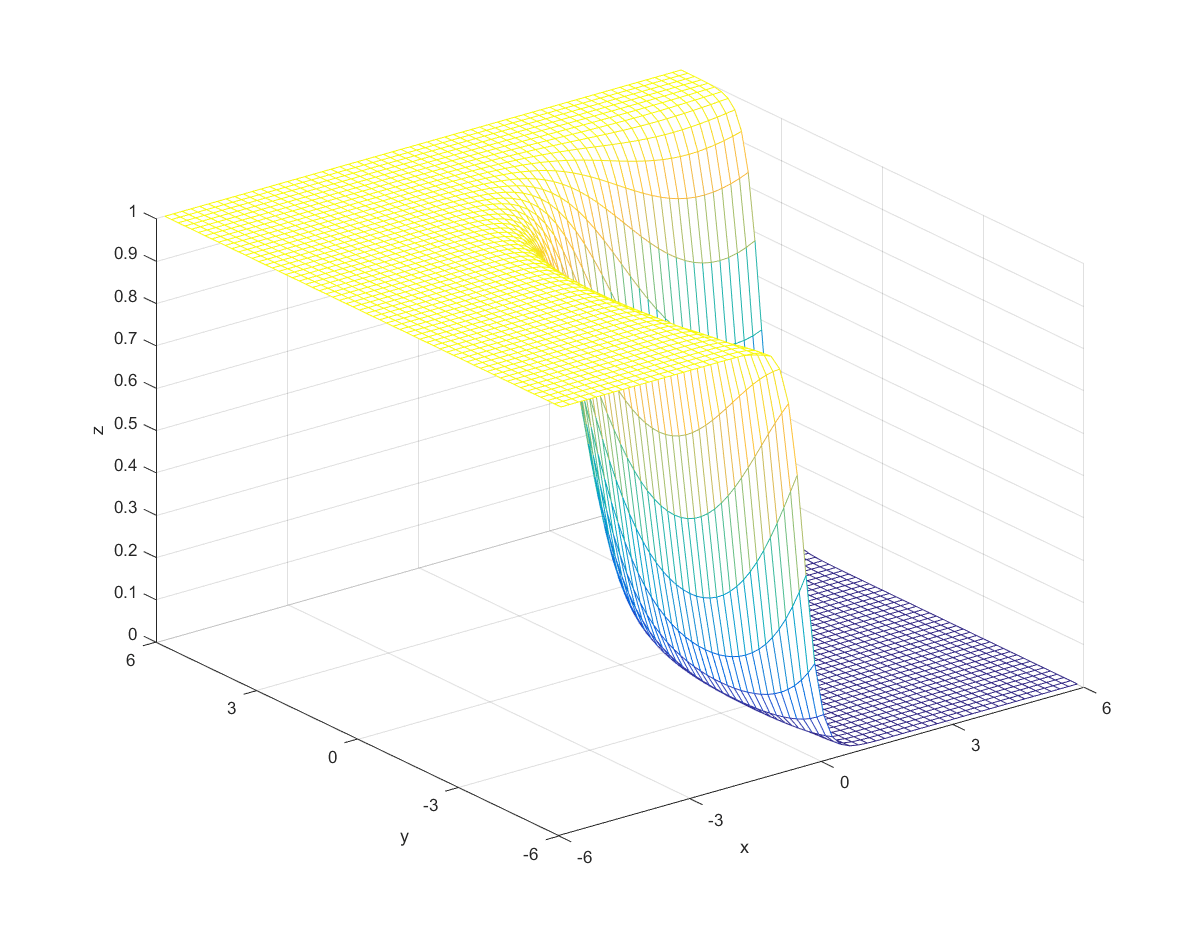
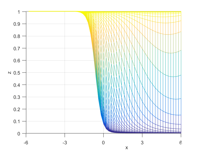
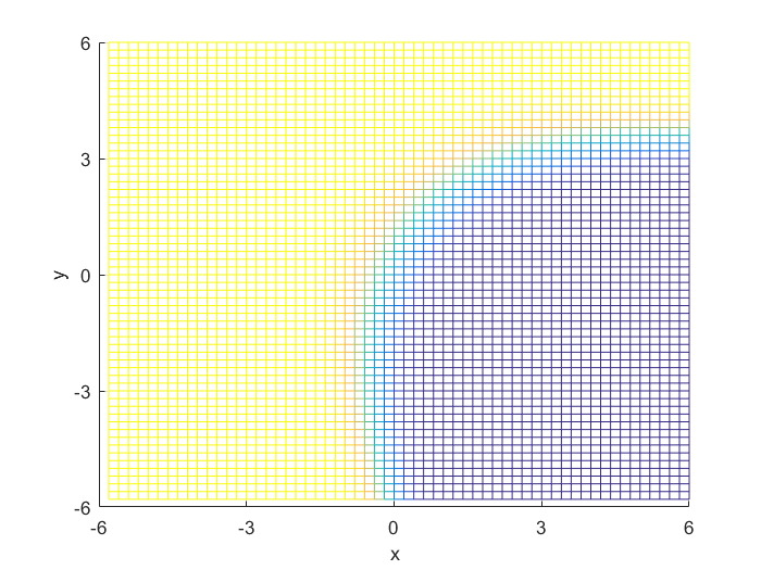
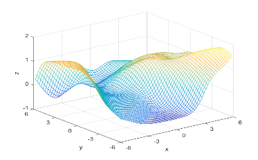
To compute the posterior probability, I started by defining the following two Gaussian distributions, they have different means and covariance matrices.

Equation

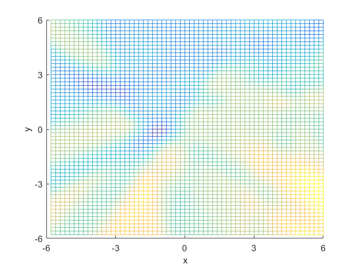
Using the definitions, I iterated over a N×N matrix, calculating the posterior probability of being in each class, with the function mvnpdf(x, m, C); To display it I chose to use a mesh because with a high enough resolution, a mesh allows you to see the pattern in the plane, and also look visually interesting. Finally, I plotted the mesh and rotated it to help visualize the class boundary. You can clearly see that the boundary is quadratic, with a sigmodal gradient.

Classification using a Feedforward Neural Network

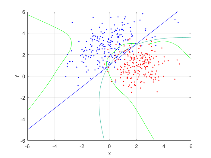
Next, I generated 200 samples with the definitions and the function mvnrnd(m, C, N);, finally partitioning it half, into training and testing sets. With the first of the sets, I trained a feed-forward neural network with 10 hidden nodes; with the second, I tested the trained neural net, and got the following errors:

Normalized mean training error: 0.0074
Normalized mean testing error: 0.0121

These values are both small, and as the testing error is marginally larger than the training error, to be expected. This shows that the neural network has accurately classified the data.

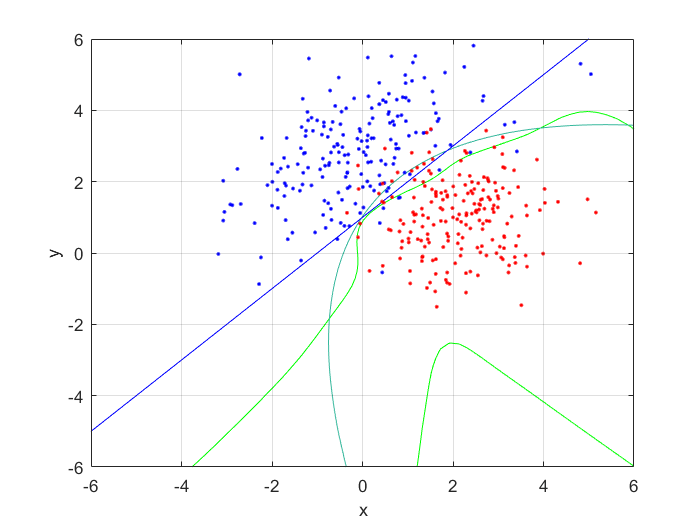
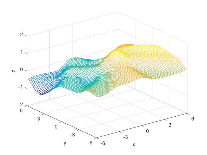
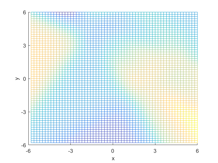
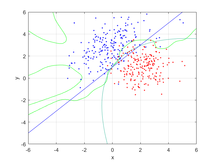
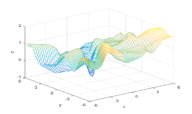
I compared the neural net contour (At 0.5) to both a linear and quadratic Bayes’ optimal class boundary. It is remarkable how significantly better Bayes’ quadratic boundary is. I blame both the low sample size, and the low number of hidden nodes. For comparison, I have also included Bayes’ linear boundary, it isn’t that bade, but still pales in comparison to the quadratic boundary. To visualize, I plotted the neural net probability mesh. It is interesting how noisy the mesh is, when compared to the Bayesian boundary.

Next, I increased the number of hidden nodes from 10, to 20, and to 50. As I increased the number of nodes I noticed that the boundary became more complex, and the error rate increased. This is because the mode nodes I added, the more I over-fitted the network. This shows that it’s incredibly important to choose the network size wisely; it’s easy to go to big! After looking at the results, I would want to pick somewhere around 5-20 nodes for this problem. I might also train it for longer.

Training Error: 0.0074 at 10 nodes, 0.0140 at 20 nodes, and 0.0153 at 50 nodes.
Testing Error: 0.0121 at 10 notes, 0.0181 at 20 nodes, and 0.0206 at 50 nodes.

Macky-Glass Predictions

I was set the task of first generating a number of samples from the Mackey-Glass chaotic time series, then using these to train and try to predict their future values using a neural net. Mackey-Glass is calculated with the equation:

Equation

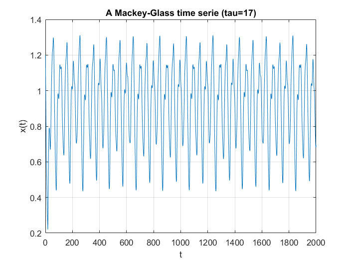
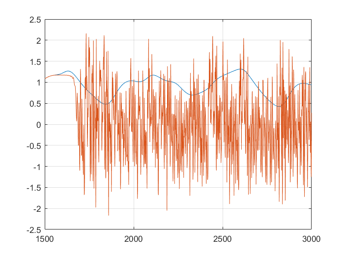
For the samples, I visited Mathworks file exchange, and downloaded a copy of Marco Cococcioni’s Mackey-Glass time series generator: https://mathworks.com/matlabcentral/fileexchange/24390. I took the code, and adjusted it to generate N=2000 samples, changing the delta from 0.1 to 1. If I left the delta at 0.1, the neural network predicted what was essentially random noise between -5 and +5. I suspect this was due to the network not getting enough information about the curve, the values given were too similar. You can see how crazy the output is in the bottom graph. Next, I split the samples into a training set of 1500 samples, and a testing set of 500 samples. This was done with p=20. I created a linear predictor and a feed-forward neural network to look at how accurate the predictions were one step ahead.

Normalized mean linear error: 6.6926×10^-4
Normalized mean neural error: 4.6980×10^-5

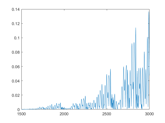
This shows that the neural network is already more accurate, a single point ahead. If you continue, feeding back predicted outputs, sustained oscillations are not only possible, the neural net accurately predicts values at least 1500 in the future. In the second and third graphs, you can notice the error growing very slowly, however even at 3000, the error is only 0.138

Financial Time Series Prediction

Using the FTSE index from finance.yahoo.com, I created a neural net predictor capable of predicting tomorrows FTSE index value from the last 20 days of data. To keep my model simpler and not over-fitted, I decided to use just the closing value, as other columns wouldn’t really affect the predictions, and just serve to over-complicate the model.

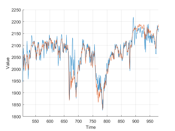
Feeding the last 20 days into the neural net produces relatively accurate predictions, however some days there is a significant difference. This is likely due to the limited amount of data, and simplicity of the model. It’s worth taking into account that the stock market is much more random and unpredictable than Mackey-Glass.

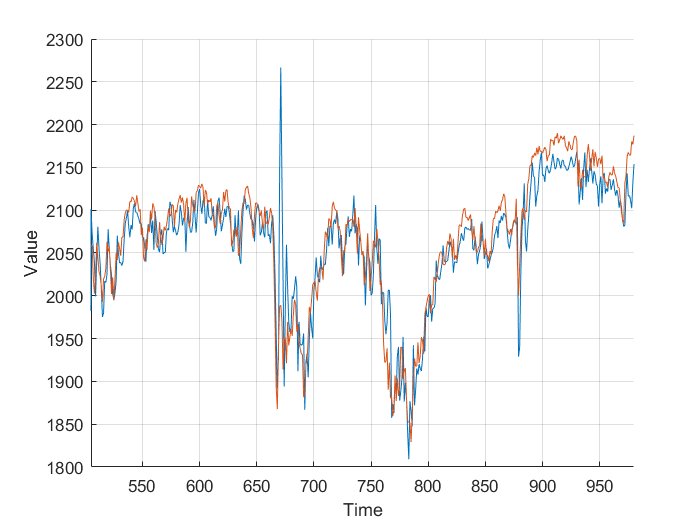
Next I added the closing volume to the neural net inputs, and plotted the predictions it made. Looking at the second graph, it’s making different predictions, which from a cursory glance, look a little more in-line.

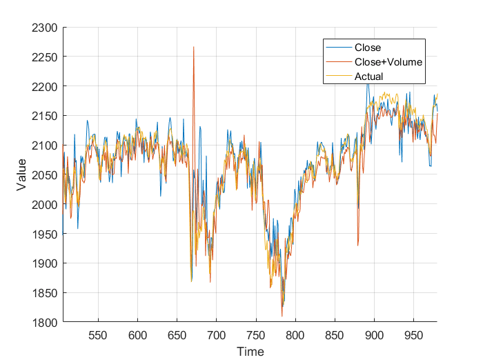
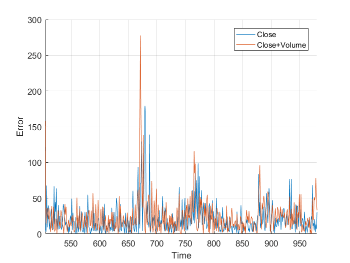
However, I wasn’t sure so I plotted them on the same axis, and, nothing really. It just looks a mess. Plotting the different errors again gives nothing but a noisy, similar mess. Finally, I calculated the total area, the area under the graph and got:

Normalized close error: 9.1066×10^5
Normalized close+volume error: 9.1180×10^5

This is nothing, a different of 0.011×10^5 is nothing when you are sampling 1000 points. It works out to an average difference of 1.131, or 0.059%. From this I, can conclude that the volume of trades has little to no effect on the closing price, at least when my neural network is concerned. All that really matters is the previous closing values.

Overall, there is certainly an opportunity to make money in the stock market, however using the model above, I wouldn’t really want to make big bets. With better models and more data, you could produce more accurate predictions, but you still must contest with the randomness of the market. I suggest further research before betting big.

Appendices

Appendix A – Neural Network Approximation Code

% Define our classes
m1 = [0;3];     m2 = [2;1];
C1 = [2 1;1 2]; C2 = [1 0;0 1];

% Generate samples
N = 200;
samples1 = mvnrnd(m1, C1, N);
samples2 = mvnrnd(m2, C2, N);

% Combine, shuffle, and partition the data
data = [samples1 zeros(N,1);samples2 ones(N,1)];
data = data(randperm(N*2), :);

% Calculation constants
probabilityResolution = 60; % Needs to be a multiple of 4
posteriorProbability  = zeros(probabilityResolution, probabilityResolution);
priorProbability1 = 0.5;
priorProbability2 = 1 - priorProbability1;

for i=1:probabilityResolution
	for j=1:probabilityResolution
		% convert 1:probabilityResolution to -6:6
		k = (i / (probabilityResolution / 2) - 1) * 6;
		l = (j / (probabilityResolution / 2) - 1) * 6;

		value1 = mvnpdf([l;k], m1, C1);
		value2 = mvnpdf([l;k], m2, C2);

		posteriorProbability(i,j) = (value1 * priorProbability1) / (value1 * priorProbability1 + value2 * priorProbability2);
	end
end

% Plot the 3d graph
mesh(posteriorProbability);
xticks([0 probabilityResolution/4 probabilityResolution/2 probabilityResolution*3/4 probabilityResolution]);
xticklabels([-6 -3 0 3 6]); xlabel('x');
yticks([0 probabilityResolution/4 probabilityResolution/2 probabilityResolution*3/4 probabilityResolution]);
yticklabels([-6 -3 0 3 6]); ylabel('y'); zlabel('z');

% Train a neural net
N = 200;
trainingData = data(1:N,:);
testingData  = data(N+1:2*N,:);

[net] = feedforwardnet(50)
[net] = train(net, trainingData(:,1:2)', trainingData(:,3)');

% Compare errors
trainingValues = zeros(N,1); testingValues  = zeros(N,1);
trainingError = 0;		   testingError  = 0;

for i=1:N
	trainingValues(i,:) = net(trainingData(i,1:2)');
	if xor(trainingValues(i,:) > 0.5, trainingData(i,3) == 1)
		trainingError = trainingError + norm(trainingValues(i,:) - 0.5);
	end
	testingValues(i,:) = net(testingData(i,1:2)');
	if xor(testingValues(i,:) > 0.5, testingData(i,3) == 1)
		testingError = testingError + norm(testingValues(i,:) - 0.5);
	end
end
trainingError/N, testingError/N

neuralMesh = zeros(probabilityResolution,probabilityResolution);
for i=1:probabilityResolution
	disp(i);
	for j=1:probabilityResolution
		% convert 1:probabilityResolution to -6:6
		k = (i / (probabilityResolution / 2) - 1) * 6;
		l = (j / (probabilityResolution / 2) - 1) * 6;
		x = [l;k];

		neuralMesh(i,j) = net(x);
	end
end

figure(1);
hold off, mesh(neuralMesh);
xticks([0 probabilityResolution/4 probabilityResolution/2 probabilityResolution*3/4 probabilityResolution])
xticklabels([-6 -3 0 3 6]); xlabel('x');
yticks([0 probabilityResolution/4 probabilityResolution/2 probabilityResolution*3/4 probabilityResolution])
yticklabels([-6 -3 0 3 6]) ylabel('y'); zlabel('z'); figure(2);
contour(linspace(-6,6,probabilityResolution), linspace(-6,6,probabilityResolution), neuralMesh,[0.5 0.5]);
xlabel('x'); ylabel('y'); hold on;

% Baye's Optimal Quadratic Class boundarys
weight1 = 2*C1'*(m2-m1),		weight2 = 2*C2'*(m2-m1)
bias1 = m1'*C1*m1 - m2'*C1'*m2, bias2   = m1'*C2*m1 - m2'*C2'*m2

grid on;
plotpc(weight1', bias1);
plotpc(weight2', bias1);
grid on; hold off;
contour(linspace(-6,6,probabilityResolution), linspace(-6,6,probabilityResolution), neuralMesh,[0.5 0.5],'Color', 'g');
hold on;
contour(linspace(-6,6,probabilityResolution), linspace(-6,6,probabilityResolution), posteriorProbability,[0.5 0.5]);
xlabel('x'); ylabel('y');
plotpc(weight1', bias1);
plotpc(weight2', bias1);
hold on;
scatter(samples1(:,1), samples1(:,2), 'b.');
scatter(samples2(:,1), samples2(:,2), 'r.');
grid on

Appendix B – Mackey-Glass Series Prediction Code

a        = 0.2;  % value for a in eq (1)
b        = 0.1;  % value for b in eq (1)
tau      = 17;   % delay constant in eq (1)
x0       = 1.2;  % initial condition: x(t=0)=x0
deltat   = 1;    % time step size (which coincides with the integration step)
sample_n = 4000; % total no. of samples, excluding the given initial condition
interval = 200;  % output is printed at every 'interval' time steps
time = 0;
index = 1;
history_length = floor(tau/deltat);
x_history = zeros(history_length, 1); % here we assume x(t)=0 for -tau <= t < 0
x_t = x0;
X = zeros(sample_n+1, 1); % vector of all generated x samples
T = zeros(sample_n+1, 1); % vector of time samples
for i = 1:sample_n+1
	X(i) = x_t;
	if (mod(i-1, interval) == 0)
		 fprintf('%4d %f\n', (i-1)/interval, x_t);
	end
	if tau == 0
		x_t_minus_tau = 0.0;
	else
		x_t_minus_tau = x_history(index);
	end
	x_t_plus_deltat = mackeyglass_rk4(x_t, x_t_minus_tau, deltat, a, b);
	if (tau ~= 0)
		x_history(index) = x_t_plus_deltat;
		index = mod(index, history_length)+1;
	end
	time = time + deltat;
	T(i) = time;
	x_t = x_t_plus_deltat;
end
hold off; plot(T(1:2000), X(1:2000));
set(gca,'xlim',[0, T(2000)]);
xlabel('t'); ylabel('x(t)');
title(sprintf('A Mackey-Glass time serie (tau=%d)', tau));
grid on

% Setup the training Matrix
N = 1500;
p = 20;
trainingMatrix = zeros(N-p,p);
trainingResult = zeros(N-p,1);
for i=1:N-p
	for j=1:p
		trainingMatrix(i,j) = X(i+j-1);
	end
	trainingResult(i) = X(i+p);
end

% Calculate the training weights
trainingWeight = inv(trainingMatrix'*trainingMatrix)*trainingMatrix'*trainingResult;

%Make predictions
O = 500;
predictionMatrix = zeros(O-p,p);
predictionResult = zeros(O-p,1);
for i=1:O-p
	for j=1:p
		predictionMatrix(i,j) = X(N+i+j-1);
	end
	predictionResult(i) = X(N+i+p);
end
predictionValues = predictionMatrix*trainingWeight;
predictionErrors = 0;
for i=1:O-p
	predictionErrors = predictionErrors + norm(predictionValues(i) - predictionResult(i));
end
predictionErrors / (O-p)

% Train the net
[net] = feedforwardnet(20)
[net] = train(net, trainingMatrix', trainingResult');
predictionErrors = 0;
for i=1:O-p
	predictionValue = net(predictionMatrix(i,:)');
	predictionErrors = predictionErrors + norm(predictionValue - predictionResult(i));
end
predictionErrors / (O-p)

% Setup
feedforwardInput = predictionMatrix(1,:);
feedforwardData = zeros(N,1);
feedforwardData(1:p) = feedforwardInput;
for i=1:N
	feedforwardValue = net(feedforwardInput');
	feedforwardInput = circshift(feedforwardInput,-1);
	feedforwardInput(p) = feedforwardValue;

	feedforwardData(i+p) = feedforwardValue;
end

hold off; plot(1501:3000, X(1501:3000));
hold on
plot(1501:3000, feedforwardData(1:1500));
grid on
feedforwardErrors = zeros(N,1);
for i=1:N
	feedforwardErrors(i) = norm(feedforwardData(i) - X(i+1500));
end
hold off; plot(1501:3000, feedforwardErrors); grid on;

Appendix C – Financial Time Series Prediction Code

% Import financial data
ftse = readtable('ftse.csv');

N = height(ftse);
ftse = table2array(ftse(:,5));
p = 20;
ftseMatrix = zeros(N-p,p);
ftseResult = zeros(N-p,1);
for i=1:N-p
	for j=1:p
		ftseMatrix(i,j) = ftse(i+j-1);
	end
	ftseResult(i) = ftse(i+p);
end
[net] = feedforwardnet(20)
[net] = train(net, ftseMatrix(1:N/2,:)', ftseResult(1:N/2)');
predictionErrors = 0;
predictionValues = zeros(N/2, 1);
for i=(N/2+1):N-p
	predictionValues(i) = net(ftseMatrix(i,:)');
	predictionErrors = predictionErrors + norm(predictionValues(i) - ftseResult(i));
end
predictionErrors / (N/2)
hold off, figure, hold on; grid on;
plot(predictionValues);
plot(ftseResult);
grid on;
xlim([505 980]);
ftse = readtable('ftse.csv');
ftse = table2array(ftse(:,5:6));
ftseMatrix = zeros(N-p,p*2);
ftseResult = zeros(N-p,1);
for i=1:N-p
	for j=1:p
	   ftseMatrix(i,j)   = ftse(i+j-1,1);
	   ftseMatrix(i,j+1) = ftse(i+j-1,2);
	end
	ftseResult(i) = ftse(i+p);
end
[net] = feedforwardnet(20)
[net] = train(net, ftseMatrix(1:N/2,:)', ftseResult(1:N/2)');
predictionErrors2 = 0;
predictionValues2 = zeros(N/2, 1);
for i=(N/2+1):N-p
	predictionValues2(i) = net(ftseMatrix(i,:)');
	predictionErrors2 = predictionErrors2 + norm(predictionValues2(i) - ftseResult(i));
end
predictionErrors2 / (N/2)
hold off, figure, hold on;
plot(predictionValues, 'DisplayName', 'Close');
plot(predictionValues2, 'DisplayName', 'Close+Volume');
plot(ftseResult, 'Displayname', 'Actual');
legend('show');
xlim([505 980]);
grid on;
xlabel('Time');
ylabel('Error');
sum(abs(ftseResult - predictionValues))
sum(abs(ftseResult - predictionValues2))

Appendix D - FTSE.csv

Data was taken from Yahoo Finance between 2012-11-30 and 2016-11-30.

A Jison, DnD-style Dice Roller Securing a Bad Blogging Platform