
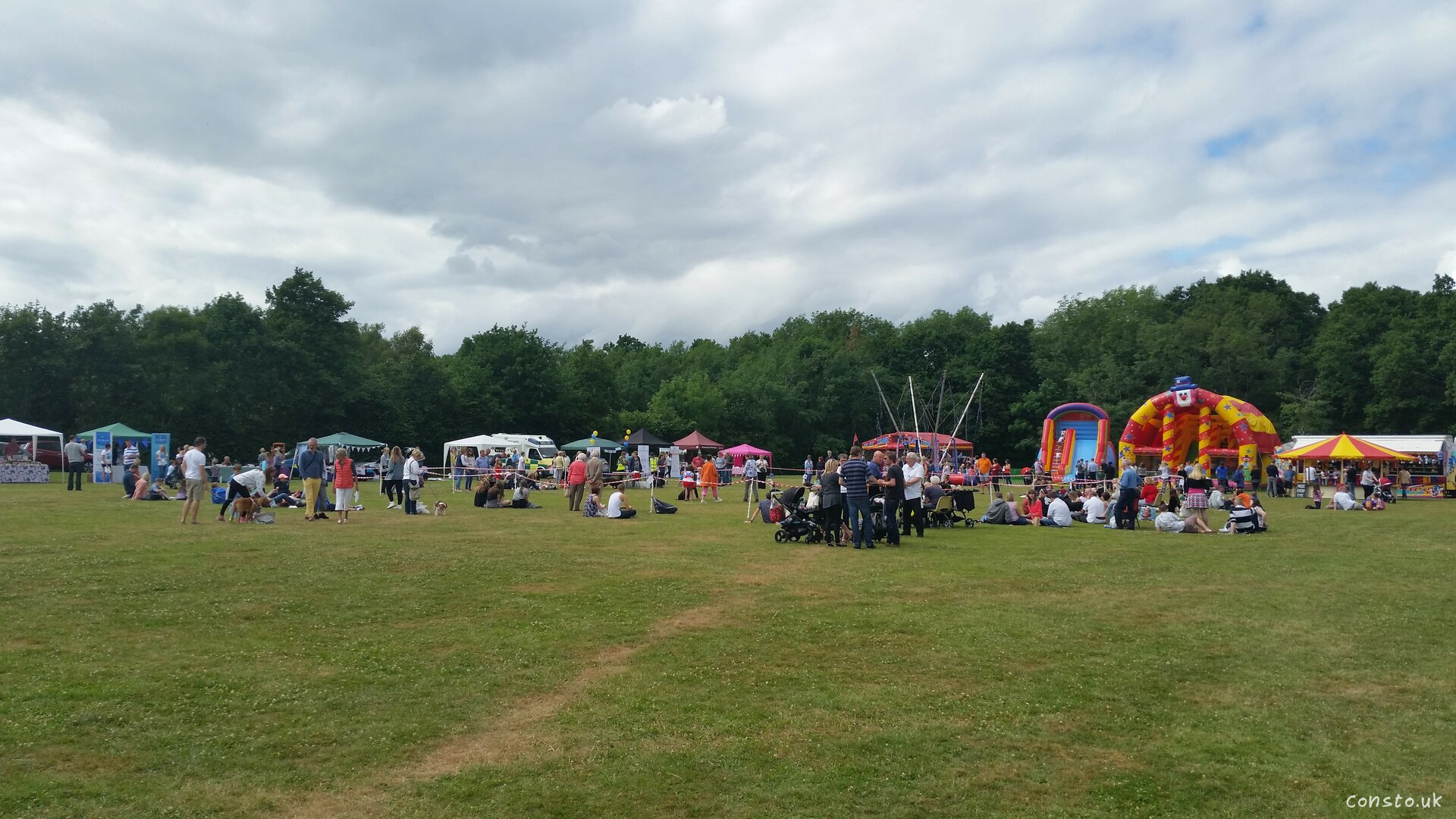
The Village Fete has Arrived Jun. 25, 2017 in Photos
It’s done, it’s over! Months in the making, my dissertation is finished an available from lect.me. My advice for future students, is to start early. Projects like these always take longer then you expect.

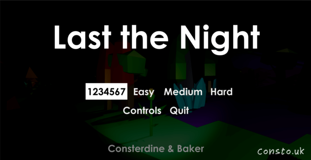
Last The Night is a procedurally generated first person survival game in which the player fights for their life after having crash landed on a mysterious, unknown planet. Armed with only a pistol, the player must fight off the various monsters inhabiting the planet, and only once the sun rises will they be safe.
With seed based world generation, there are literally millions of planets to explore with no two being the same, and with the addition of Easy, Medium and Hard difficulties, advanced players can challenge themselves whilst beginners can get a feel for the game. Last The Night features 17 different types of monsters, keeping the player guessing at all times.
A student game created at the University of Southampton by Matthew Consterdine and Ed Baker. Do you think you’re brave enough to last the night?

Using your flame-thrower, wrack up points and burn the forest down. Single player, play with a mouse/keyboard or Xbox 360 controller. A student game created at the University of Southampton during the Southampton Code Dojo. Burn down everything!.
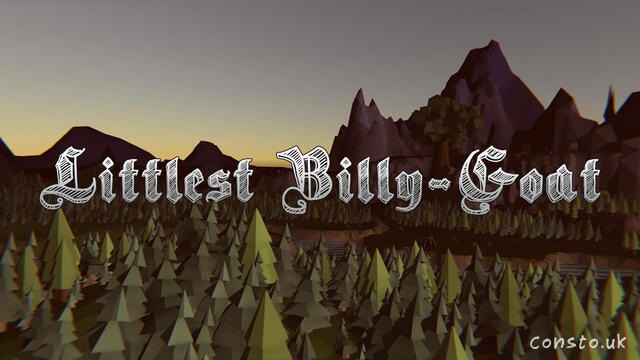
A fully narrated re-telling of the fairy tale classic. Single player, play with a mouse/keyboard or Xbox 360 controller. A student game created at the University of Southampton by Matthew Consterdine and Jeff Tomband. Download and play.
Having previously created games in my spare time and in competitions, I chose to team up with three different partners to create games focusing on gameplay, narrative experiences, and innovative technology using Unity. It was hard, took a lot of work, but in the end it was one of the most satisfying modules I ever took at University. Shout out to Rikki Prince, Dave Millard, and Tom for running such and excellent module.
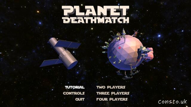
A fast paced, Quake inspired, local multi-player, little planet deathmatch infinite arena shooter. Hone your skills, then compete against your friends to see who can dominate the playing field. Supports up to 4 player split-screen, bring an Xbox controller. A student game created at the University of Southampton by Matthew Consterdine and Ollie Steptoe.
Featuring a number of classic weapons:
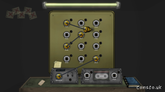
A Paper’s-Please style telephony simulation created at the Southampton Game Jam. Play here.
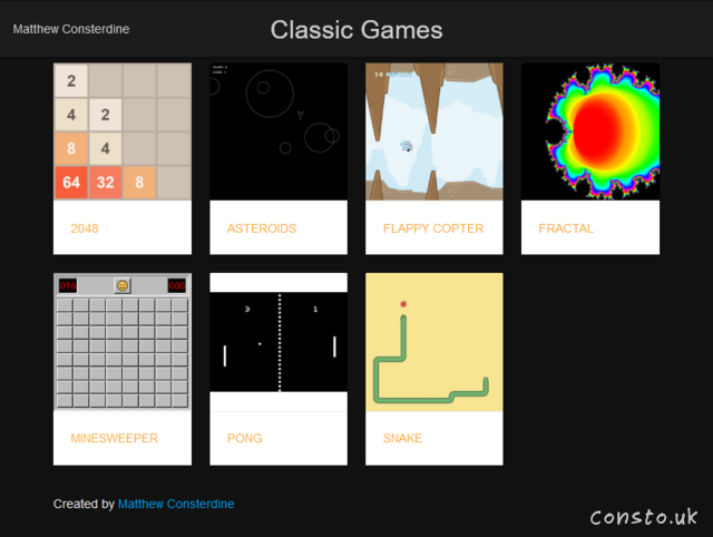
I’ve put together a HTML5 recreation of several classic games. Play online.
I was tasked with securing $BloggingPlatform. Here are my findings.
I decided to investigate Machine Learning using MATLAB.
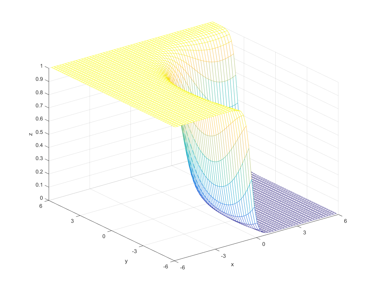
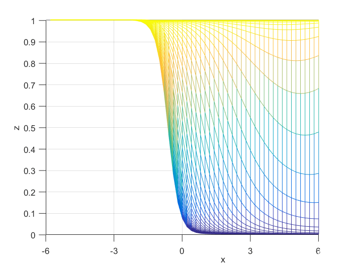
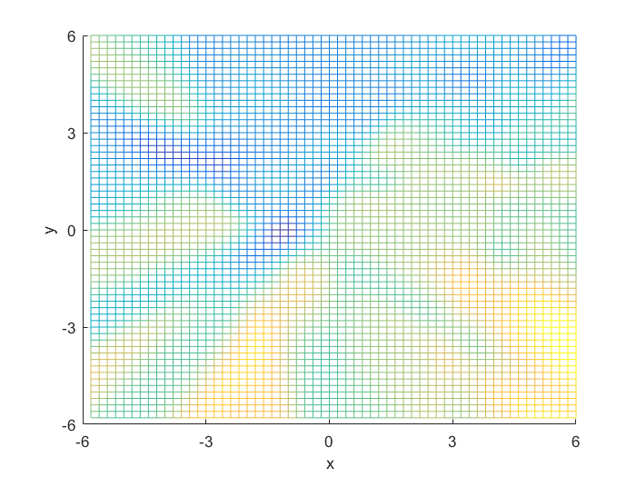
To compute the posterior probability, I started by defining the following two Gaussian distributions, they have different means and covariance matrices.

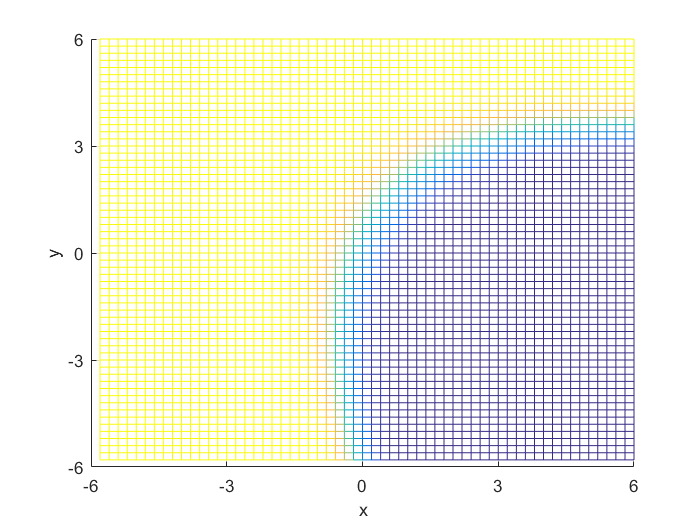
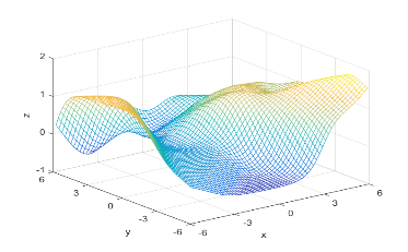
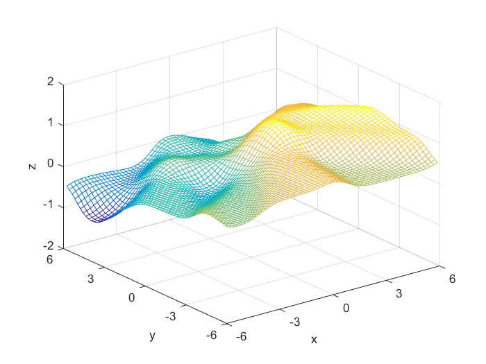
Using the definitions, I iterated over a N×N matrix, calculating the posterior probability of being in each class, with the function mvnpdf(x, m, C); To display it I chose to use a mesh because with a high enough resolution, a mesh allows you to see the pattern in the plane, and also look visually interesting. Finally, I plotted the mesh and rotated it to help visualize the class boundary. You can clearly see that the boundary is quadratic, with a sigmodal gradient.
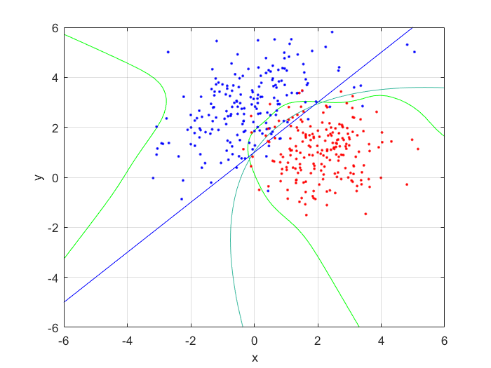
Next, I generated 200 samples with the definitions and the function mvnrnd(m, C, N);, finally partitioning it half, into training and testing sets. With the first of the sets, I trained a feed-forward neural network with 10 hidden nodes; with the second, I tested the trained neural net, and got the following errors:
These values are both small, and as the testing error is marginally larger than the training error, to be expected. This shows that the neural network has accurately classified the data.
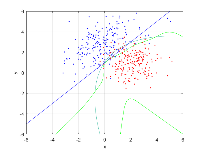

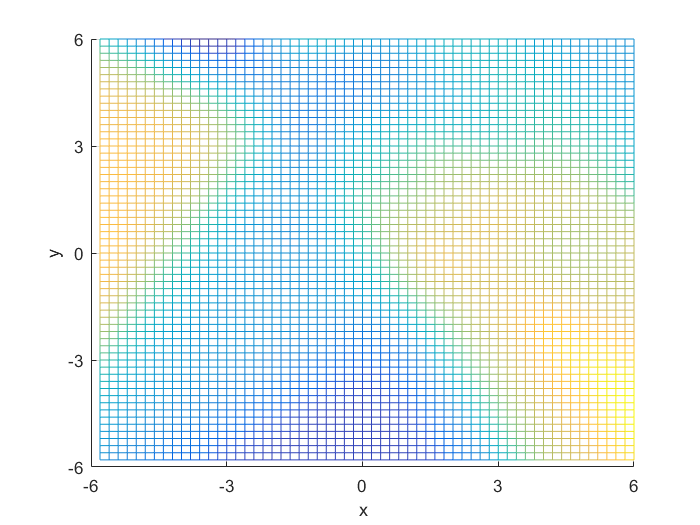
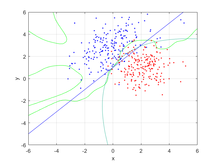
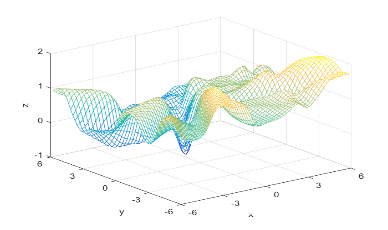
I compared the neural net contour (At 0.5) to both a linear and quadratic Bayes’ optimal class boundary. It is remarkable how significantly better Bayes’ quadratic boundary is. I blame both the low sample size, and the low number of hidden nodes. For comparison, I have also included Bayes’ linear boundary, it isn’t that bade, but still pales in comparison to the quadratic boundary. To visualize, I plotted the neural net probability mesh. It is interesting how noisy the mesh is, when compared to the Bayesian boundary.
Next, I increased the number of hidden nodes from 10, to 20, and to 50. As I increased the number of nodes I noticed that the boundary became more complex, and the error rate increased. This is because the mode nodes I added, the more I over-fitted the network. This shows that it’s incredibly important to choose the network size wisely; it’s easy to go to big! After looking at the results, I would want to pick somewhere around 5-20 nodes for this problem. I might also train it for longer.
I was set the task of first generating a number of samples from the Mackey-Glass chaotic time series, then using these to train and try to predict their future values using a neural net. Mackey-Glass is calculated with the equation:

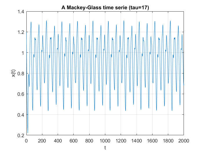
For the samples, I visited Mathworks file exchange, and downloaded a copy of Marco Cococcioni’s Mackey-Glass time series generator: https://mathworks.com/matlabcentral/fileexchange/24390. I took the code, and adjusted it to generate N=2000 samples, changing the delta from 0.1 to 1. If I left the delta at 0.1, the neural network predicted what was essentially random noise between -5 and +5. I suspect this was due to the network not getting enough information about the curve, the values given were too similar. You can see how crazy the output is in the bottom graph. Next, I split the samples into a training set of 1500 samples, and a testing set of 500 samples. This was done with p=20. I created a linear predictor and a feed-forward neural network to look at how accurate the predictions were one step ahead.

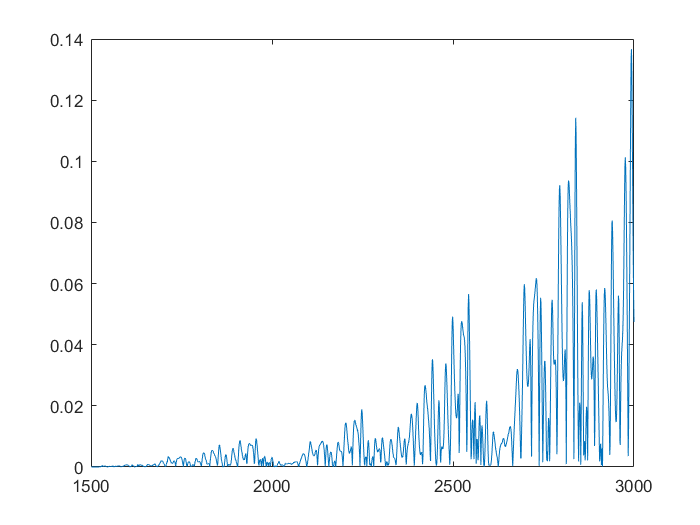
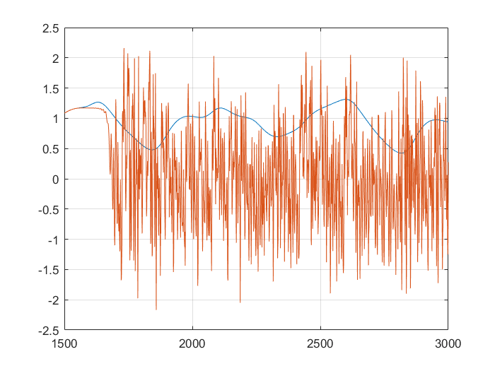
This shows that the neural network is already more accurate, a single point ahead. If you continue, feeding back predicted outputs, sustained oscillations are not only possible, the neural net accurately predicts values at least 1500 in the future. In the second and third graphs, you can notice the error growing very slowly, however even at 3000, the error is only 0.138
Using the FTSE index from finance.yahoo.com, I created a neural net predictor capable of predicting tomorrows FTSE index value from the last 20 days of data. To keep my model simpler and not over-fitted, I decided to use just the closing value, as other columns wouldn’t really affect the predictions, and just serve to over-complicate the model.
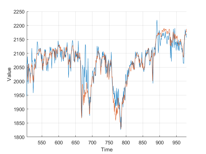
Feeding the last 20 days into the neural net produces relatively accurate predictions, however some days there is a significant difference. This is likely due to the limited amount of data, and simplicity of the model. It’s worth taking into account that the stock market is much more random and unpredictable than Mackey-Glass.
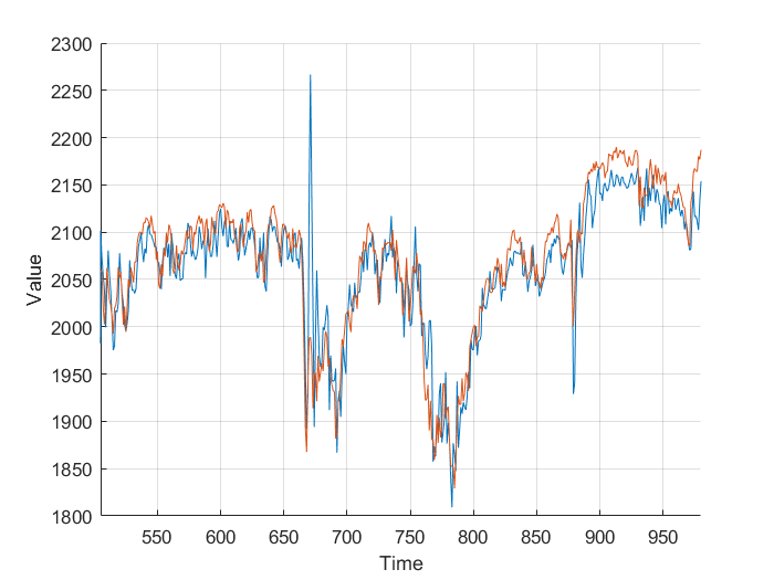
Next I added the closing volume to the neural net inputs, and plotted the predictions it made. Looking at the second graph, it’s making different predictions, which from a cursory glance, look a little more in-line.
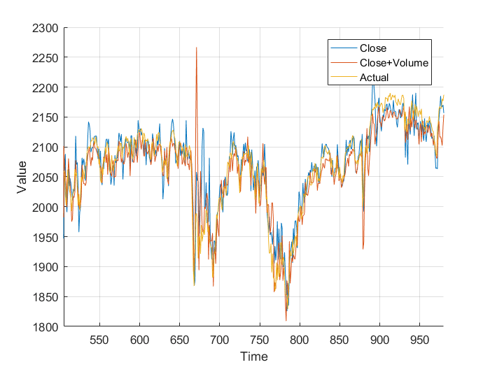
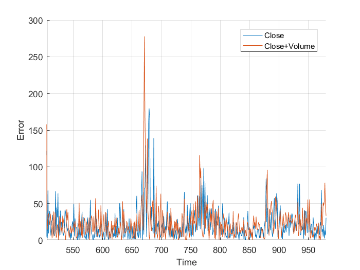
However, I wasn’t sure so I plotted them on the same axis, and, nothing really. It just looks a mess. Plotting the different errors again gives nothing but a noisy, similar mess. Finally, I calculated the total area, the area under the graph and got:
This is nothing, a different of 0.011×10^5 is nothing when you are sampling 1000 points. It works out to an average difference of 1.131, or 0.059%. From this I, can conclude that the volume of trades has little to no effect on the closing price, at least when my neural network is concerned. All that really matters is the previous closing values.
Overall, there is certainly an opportunity to make money in the stock market, however using the model above, I wouldn’t really want to make big bets. With better models and more data, you could produce more accurate predictions, but you still must contest with the randomness of the market. I suggest further research before betting big.